


Demystifying Neural Network Architecture for Business and Product Leaders
Using "Tensorflow Playground", an interactive product sandbox, to visualize and experiment with neural networks.

Neural networks are at the heart of most AI-driven innovations, including the latest craze around Generative AI / ChatGPT. Yet, their inner workings are often not well understood by many. With Business Leaders and Product Managers as the primary target audience, the intent of this article is to provide a quick and comprehensive overview of the inner workings of a multi-layer neural network. Using TensorFlow Playground — an interactive, web-based tool — we will demystify how the neural networks operate and highlight their practical applications on 4 sample datasets with increasing complexity.
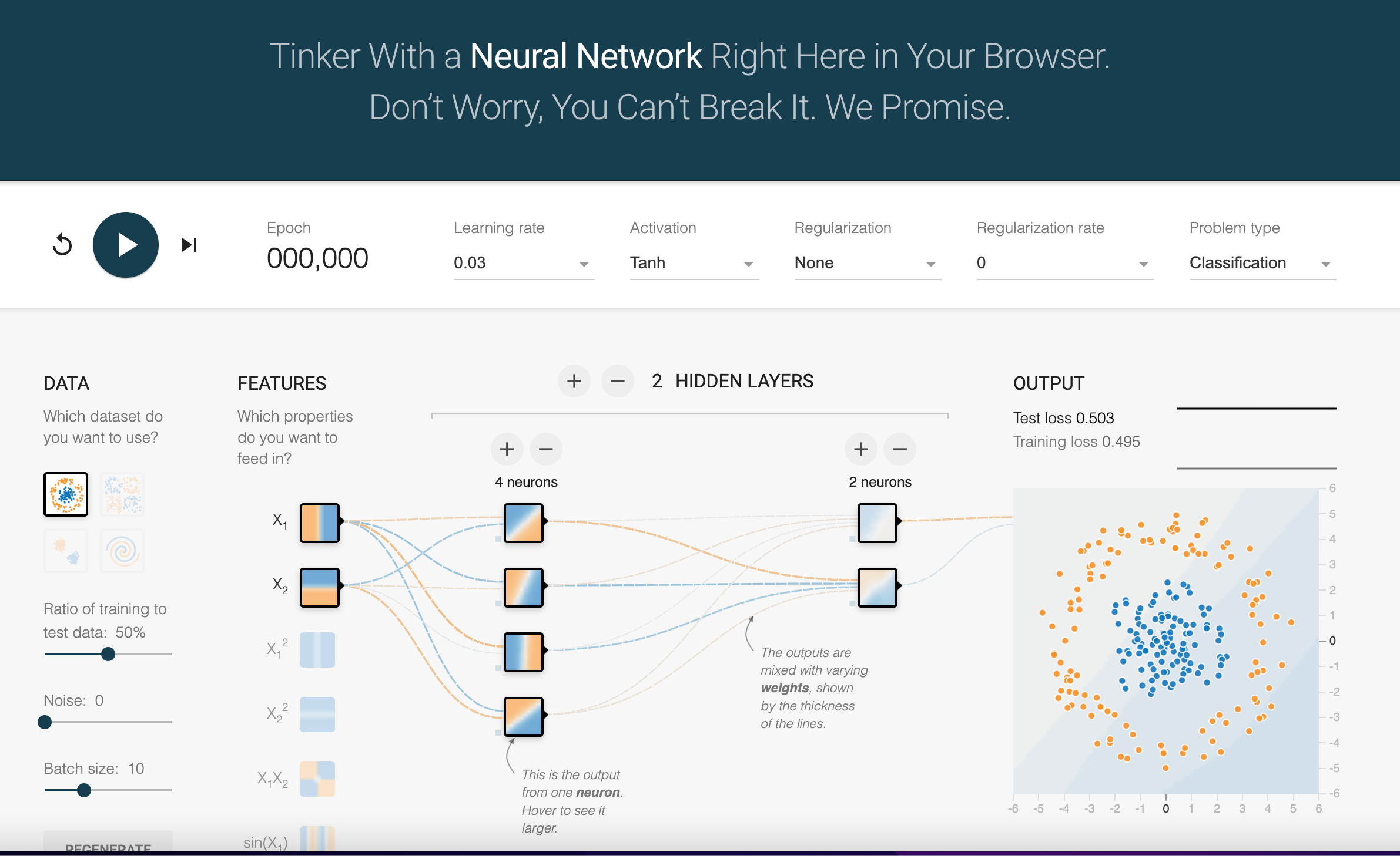
TensorFlow Playground, one of the best product sandbox (aka, product playground), is an interactive platform designed to visualize and experiment with neural networks. It allows users to interactively modify parameters, observe decision boundaries, and monitor performance metrics in real time. Whether you’re a beginner or a seasoned AI enthusiast, TensorFlow Playground serves as a valuable resource for deepening your understanding of these powerful algorithms.

Anatomy of a Multi-Layer Neural Network
From Single Neurons to Networks
At the core of any neural network is the neuron, a mathematical function inspired by biological neurons. A single neuron takes input values, applies weights and a bias (for example, Z = aX1 + bX2 + cX3 + d ; where X1, X2 and X3 are inputs; a, b and c are weights and d is the bias) and passes the result, Z above, through an activation function to produce an output for the neuron. Mathematically, this process can be expressed as:
Output = Activation (Σ(Weights × Inputs) + Bias)
Inputs: The raw data values, such as features from a dataset.
Weights: Determine the importance of each input.
Bias: An offset value to adjust the output independent of inputs.
Activation Function: Introduces non-linearity, enabling the neuron to learn complex patterns. Without it, the network would behave as a linear model, incapable of solving non-linear problems.

Building Multi-Layer Networks
In a multi-layer neural network, neurons are organized into layers:
Input Layer: Directly receives raw data.
Hidden Layers: Perform transformations to extract features and patterns.
Output Layer: Provides final predictions or classifications.
Each layer processes the information and passes its outputs to the next layer through forward propagation. Adding layers allows the network to learn hierarchical representations of data—from simple to complex patterns. Deciding how many layers and how many neurons in each layer is a design decision based on the problem/s being solved.

The Goal of Training a Neural Network
The primary goal of training a multi-layer neural network is to determine the optimal values for weights and biases (e.g. a, b, c and d above for every neuron and layer) to minimize the loss for a particular dataset. This optimization ensures that the network’s predictions are as close as possible to the actual outputs.
Note that we are given the input dataset X1, X2, X3 etc. and use a neural network to determine the eventual output Y. However, during training phase of the neural network, we use training dataset which has the inputs X1, X2, X3 etc. as well as the expected output Y which is critical to training the multi-layer neural network.
During training:
Forward propagation computes the predictions.
The loss function quantifies the error between predictions and actual outputs.
Backpropagation adjusts weights and biases iteratively to reduce this error.
By continuously refining these parameters, the network learns to generalize patterns from the data, improving its performance on unseen examples.
The Universal Approximation Theorem
The universal approximation theorem states that a neural network with at least one hidden layer containing a sufficient number of neurons can approximate any continuous function. This foundational concept underscores why multi-layer networks are so powerful: they can model highly complex relationships between inputs and outputs.
Loss Function and Backpropagation
The performance of a neural network is measured using a loss function, which quantifies the difference between predicted and actual outputs. Examples include Mean Squared Error (MSE) for regression (to predict a value) and Cross-Entropy Loss for classification.

To improve performance, the network iteratively adjusts its weights and biases through backpropagation (over many passes through training data set):
Compute gradients of the loss function relative to each parameter.
Update parameters using an optimization algorithm (e.g., Stochastic Gradient Descent or Adam).
This iterative process continues until the network minimizes the loss function, producing an optimized model.
Exploring TensorFlow Playground
Key Parameters
TensorFlow Playground provides an intuitive interface to explore neural network configurations. Each parameter plays a crucial role in model behavior:
Neurons per Layer: Defines the number of processing units in a hidden layer. More neurons capture complex patterns but risk overfitting.
Number of Hidden Layers: Determines the depth of the network. Additional layers allow for hierarchical learning.
Activation Functions: Non-linear transformations applied at each neuron. Options include ReLU (simple and efficient), Tanh (smooth gradients), and Sigmoid (useful for probabilities).
Learning Rate: Controls the speed of parameter updates. High rates risk overshooting; low rates may converge slowly.
Regularization Rate: Penalizes large weights to prevent overfitting. L1 regularization encourages sparsity, while L2 discourages large parameter values.
Batch Size: The number of samples processed simultaneously during training. Smaller batches provide detailed updates but require more computation.
Epochs: The number of times the entire dataset is passed through the network. More epochs can improve learning but risk overfitting.
Data Features: Specifies input variables (e.g., X1, X2). Selecting relevant features improves model performance.
Interactive Experimentation
TensorFlow Playground allows users to visualize decision boundaries, track loss and accuracy, and experiment with configurations. For example:
Observe how changing the number of neurons impacts decision boundaries.
Compare the performance of different activation functions on the same dataset.
Experiment with regularization to understand its impact on generalization.
Guided Exercises
Exercise 1: Understanding Overfitting
Select the "circle" dataset.
Start with one hidden layer containing two neurons and train the model for 100 epochs.
Add more neurons (e.g., increase to 8) and retrain. Observe the decision boundary.
Enable L2 regularization and compare results. Reflect on how regularization helps reduce overfitting.
Exercise 2: Exploring Activation Functions
Select the "spiral" dataset.
Create a network with two hidden layers, each with four neurons.
Train the model using the Tanh activation function and observe the performance.
Switch to ReLU and retrain. Compare decision boundaries and accuracy.
Analyze which activation function performs better and why.
Exercise 3: Optimizing Learning Rate
Select the "XOR" dataset.
Use one hidden layer with eight neurons.
Set the learning rate to 0.5 and train for 100 epochs. Note the behavior of the loss function.
Reduce the learning rate to 0.01 and retrain. Observe changes in the loss curve and decision boundary.
Experiment with intermediate learning rates to find an optimal balance.
Key Takeaways
Understand Model Complexity: More layers and neurons can improve performance but risk overfitting.
Importance of Data Quality: Clean, relevant data is critical for effective training.
Experimentation is Essential: Neural networks often require iterative tuning.
Visualization Tools Accelerate Learning: Use TensorFlow Playground to simplify complex concepts and communicate them effectively.